20 Basic Excel Formulas You Must Know
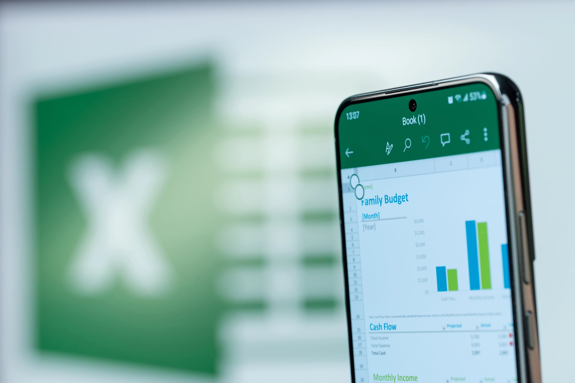
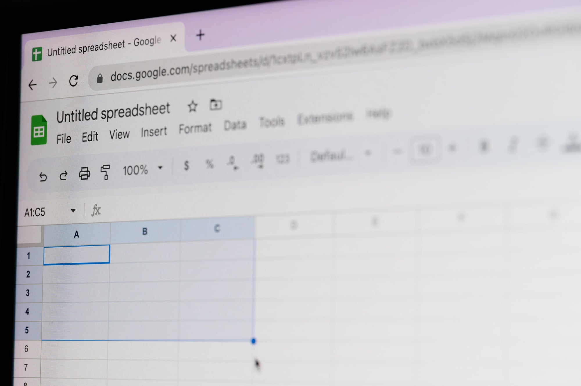
Excel becomes way more than just rows and columns once you get how its formulas work. When handling expenses, checking sales figures, or keeping an eye on deadlines, those built-in tools do the tough math instead of making you figure it out by hand.
Picking up these skills doesn’t mean learning fancy jargon; rather, it’s like having the right gadget ready whenever a certain task pops up. Check out this lineup of 20 must-know Excel formulas – perfect for anyone who uses spreadsheets regularly.
SUM
The SUM formula piles up values across a group of cells, so you don’t have to tally them by hand. Just enter =SUM(A1:A10) to grab all figures from A1 right down to A10.
It also handles separate cells – say =SUM(A1,B5,C3) – letting you mix digits however suits your setup.
AVERAGE
Need the middle number from a list? AVERAGE handles it fast.
Try =AVERAGE(B2:B20) – it totals up everything there, then splits it by how many numbers show up. Skips blanks or words without issue, zeroing in on actual digits for a solid result.
COUNT
Imagine you’ve got a bunch of cells – some filled, some empty. COUNT tells you exactly how many hold actual numbers.
Try typing =COUNT(C1:C50), hit enter, and boom – you see only the count of number-filled spots, ignoring any blank spaces or words stuck in there. This trick comes in handy if you’re double-checking your real data size before doing bigger math stuff.
COUNTA
Instead of just numbers, COUNTA picks up every non-blank cell – text, dates, anything. Use =COUNTA(D1:D100), and it tallies all entries there, no matter what’s inside.
It’s super handy if you’re checking replies, headcounts, or situations where having info is key, regardless of format.
MAX and MIN
MAX grabs the biggest number from a list, whereas MIN picks out the smallest – showing you right away where your data stands at both ends. Use =MAX(E1:E30) when hunting for the top figure, or swap it with =MIN(E1:E30) to spot the lowest one.
They skip over words and blank spots, zeroing in only on actual numbers instead.
IF

The IF function runs a test to see what’s true or false, then gives one result for yes and another for no. Try typing =IF(F2>100,’High’,’Low’) – it shows ‘High’ when F2 is bigger than 100; otherwise it says ‘Low.’
Once you get this down, it opens the door to smarter, branching spreadsheet setups.
SUMIF

SUMIF pulls together numbers matching one condition, mixing summing action with if-style checks. When you use =SUMIF(G1:G50,’>500′,H1:H50), it grabs entries from H1:H50 only if the related spot in G1:G50 is bigger than 500.
This works well when counting up revenue past a limit or costs tied to a certain type.
COUNTIF

If you’ve got to tally up cells meeting one particular rule, COUNTIF does it quick. Try typing =COUNTIF(I1:I40,’Complete’) to see how many times ‘Complete’ shows up from I1 to I40.
Another option? Use signs like greater than – say, =COUNTIF(J1:J40,’>75′) – to track down numbers over 75 in column J.
AVERAGEIF

AVERAGEIF grabs the average from certain cells based on a rule you set, tossing aside anything that doesn’t match before doing math. For instance, =AVERAGEIF(K1:K60,’>=60′,L1:L60) works out the numbers in L1:L60 just when K1:K60 hits 60 or more.
So instead of sifting through everything by hand, it lets you dig into specific chunks right away.
VLOOKUP

VLOOKUP hunts down a match in the leftmost column of your data, spitting out info from a different column on that same line. Take =VLOOKUP(M2,A1:D100,3,FALSE): it scans column A for whatever’s in cell M2 before grabbing what’s sitting three columns over.
When you need to link up entries across separate lists – or pull details from a master chart – this function gets the job done without fuss.
HLOOKUP

HLOOKUP does something similar to VLOOKUP – only it scans left to right along rows rather than top to bottom through columns. Try typing =HLOOKUP(N2,A1:Z5,3,FALSE) if you want to locate N2 within the first row and grab what’s sitting three rows beneath it.
You’ll find this function handy when your data stacks labels up front and values underneath them.
INDEX and MATCH

INDEX paired with MATCH gives you a smarter way to look things up compared to VLOOKUP – no need to worry about which column comes first. Instead of being stuck left-to-right, it checks values anywhere in your range.
Take this example: =INDEX(B1:B50,MATCH(P2,A1:A50,0)). It spots where P2 shows up in A1:A50 then grabs the matching entry from B1:B50 right across. When your search column sits somewhere on the right side, this duo still gets the job done.
CONCATENATE or CONCAT

Putting together text from different spots? Use CONCATENATE – or try CONCAT if you like newer stuff – it pulls info from several cells into one. Type something like =CONCAT(Q2,’ ‘,R2), that smushes Q2 and R2 with a blank gap in the middle.
Works great when linking first names with last ones, tossing address parts into a single box, or building tags from bits of scattered details.
LEFT, RIGHT, and MID
These text tools pull out parts of cell content by where letters sit. LEFT takes symbols from the start – like =LEFT(S2,5) grabbing five up front; RIGHT snags stuff from the tail end; while MID yanks a chunk from somewhere inside, say =MID(S2,3,4), kicking off at position three and going four deep.
You’d use these when splitting info – think pulling area codes off phone digits or plucking dates hidden in words.
LEN
LEN checks how long the text is inside a cell – spaces and symbols included. Using =LEN(T2) gives back the total number of letters, numbers, or signs in cell T2.
It’s useful when you need to confirm entries are correct, say 5-digit postal codes or making sure item IDs fit a certain size.
TRIM
TRIM gets rid of extra blank spots in your text – just one space stays between words. Try =TRIM(U2) when imported info comes cluttered with gaps at the start, end, or more than one space mid-sentence.
This trick isn’t fancy, yet it makes text consistent so searches or matches work right.
TODAY and NOW

TODAY shows today’s date, whereas NOW includes the exact time too – both refresh every time you load the sheet. Use =TODAY() if you only need the day, but go with =NOW() when seconds matter.
They’re handy for figuring out someone’s age, counting down to due dates, or marking when a report came together. Each update happens live once the file opens.
DATE
The DATE function pulls together a date using individual numbers for year, month, and day – letting you set the exact date you want. Try =DATE(2025,12,31), it turns those numbers into Dec 31, 2025, piece by piece.
Handy if your info spreads dates over different columns – or better yet, when pulling dates from results of earlier math.
ROUND, ROUNDUP, and ROUNDDOWN

These formulas decide how Excel manages decimals when it calculates stuff. For instance, ROUND follows normal rounding – like =ROUND(V2,2) – to hold just two digits after the point; on the flip side, ROUNDUP pushes numbers higher no matter what the decimal is.
Meanwhile, ROUNDDOWN drops them lower every single time, even if the number’s close to going up. Together, they help money math show results exactly as precise as required.
TEXT
TEXT turns digits into words using your chosen layout – this lets you decide exactly how figures show up. Try =TEXT(W2,’$0.00′) to see W2 look like cash with cents included; on the flip side, =TEXT(X2,’MMMM DD, YYYY’) changes dates so they read ‘January 15, 2025’.
Works great if you’re mixing neat-looking numbers with written bits in summaries or tags.
Making Excel Work for You
These formulas make up the basic tools that change Excel from just a number tracker into something way more powerful for digging into data. After using them with actual numbers, you’ll begin noticing how stacking them together can handle boring repeat jobs or uncover trends you didn’t catch before.
What matters most isn’t remembering each tiny rule, but knowing which one fits the task right now.
More from Go2Tutors!

- The Romanov Crown Jewels and Their Tragic Fate
- 13 Historical Mysteries That Science Still Can’t Solve
- Famous Hoaxes That Fooled the World for Years
- 15 Child Stars with Tragic Adult Lives
- 16 Famous Jewelry Pieces in History
Like Go2Tutors’s content? Follow us on MSN.